A complete data science pipeline applied to computational immunology
When a new pathogen emerges, the scientific community faces a question that is as urgent as it is complex: which part of the virus should a vaccine target? A pathogen can have dozens of proteins, but not all of them are equally visible to the immune system. Identifying the most promising candidates has historically been a slow and costly process that depends on specialized lab infrastructure and years of experimentation.
In 2024, Demis Hassabis and John Jumper were awarded the Nobel Prize in Chemistry for AlphaFold, an AI system capable of predicting a protein's three-dimensional structure from its amino acid sequence — something that previously required years of X-ray crystallography. The message is unmistakable: computation is no longer a complement to biology, it's one of its pillars.
AiGenix: Antigen Predictor sits at that same intersection. It's an educational project that builds, from scratch and using public data, a classifier capable of estimating the probability that a viral protein is antigenic — that is, that the human immune system detects it and responds to it. It doesn't aim to compete with large computational immunology models. It aims for something more valuable for someone just starting out: to demonstrate that with Python, curiosity, and persistence, you can tackle a real biological problem.
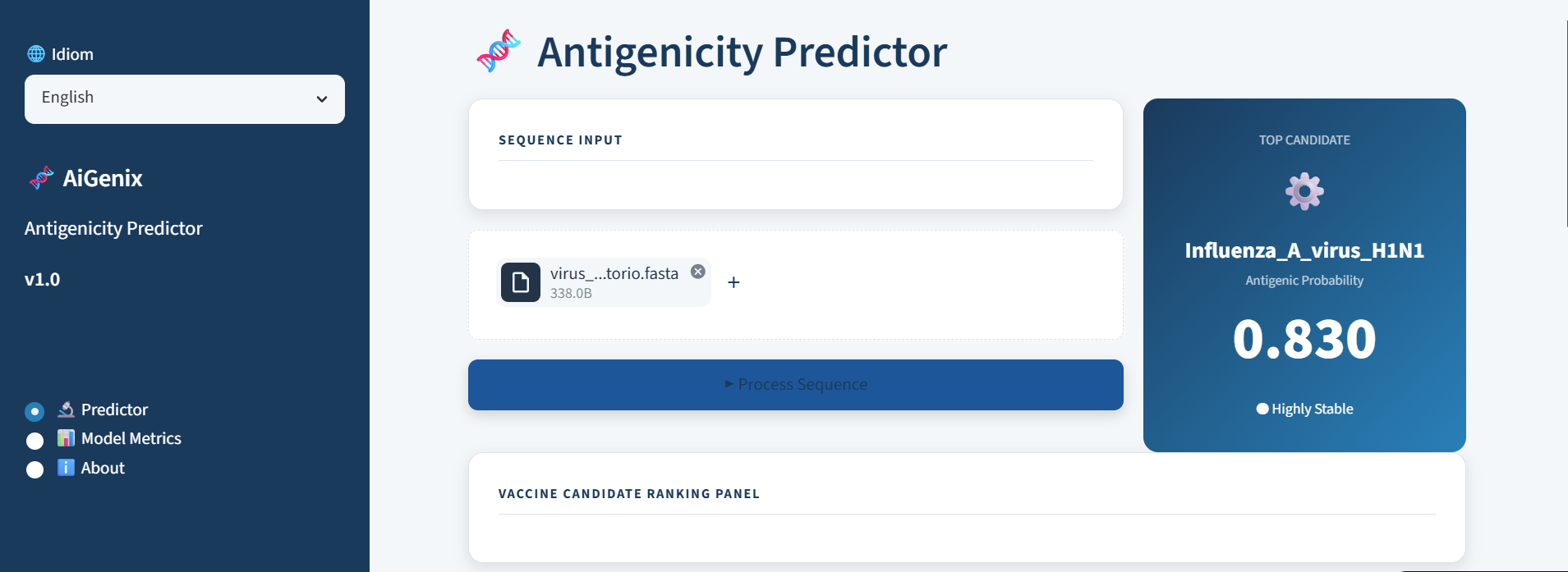
Figure 1: AiGenix's user interface. A functional dashboard built with Streamlit that lets researchers upload viral proteomes and instantly get a prioritized ranking of the most promising candidates.
Key concepts before we start
To follow the article without getting lost, it helps to be clear on the conceptual chain that connects biology to machine learning.
Protein. Proteins are the molecular machines of living organisms. They're encoded in genes and are responsible for almost everything that happens in a cell — from physical structure to chemical signaling. Viruses are also made primarily of proteins: the SARS-CoV-2 Spike protein, for example, is the key the virus uses to enter our cells.
Epitope. The immune system doesn't recognize whole proteins: it recognizes fragments. An epitope is a small segment of a protein — typically between 8 and 20 amino acids — that the immune system learns to identify as foreign. They are, in essence, the molecular fingerprints of the pathogen.
Antigenicity. A protein is antigenic if it contains epitopes that trigger an immune response. It's important to distinguish it from immunogenicity — antigenicity is the ability to be recognized; immunogenicity is the ability to provoke a complete and lasting response. This project focuses on the former: predicting whether a protein will be visible to the immune system.
IEDB. The Immune Epitope Database is the world's largest repository of experimental epitope results. It contains hundreds of thousands of real lab assays — protein fragments that were tested in the lab, with their documented outcome: Positive, Negative, Positive-High, etc. It's the source of truth for our project.
With these concepts in mind, we can describe the central question that guides the whole project: can a machine learning model, trained on existing experimental data, estimate the probability that a protein is antigenic by looking only at its amino acid sequence?
The pipeline: overview
The project is organized into five notebooks that form a sequential pipeline. Each one takes the previous one's output and produces something new:
| Step | Notebook | Output | Size |
|---|---|---|---|
| 1 | download_files | Raw data | 3.9 GB |
| 2 | 00_acquisition | Filtered CSV | 29 MB |
| 3 | 01_exploration | protein_labels | 1,365 proteins |
| 4 | 02_construction | dataset.csv | 1,310 proteins |
| 5 | 03_model | model.pkl | RF + metadata |
Notebook 0: Downloading the raw data
The first step is the most mechanical and the most critical: getting the data. IEDB offers its full exports as compressed CSV files. We download three files:
tcell_full_v3.csv— T-cell response assays (~1.3 GB uncompressed)bcell_full_v3.csv— B-cell and antibody response assays (~2.6 GB)antigen_full_v3.csv— antigen catalog with metadata
The notebook automates this download with a function that fetches the ZIP from IEDB's public URL, extracts it into data/raw/, and removes the compressed file. There's no data transformation here — just making sure the raw material is available locally. The result is roughly 3.9 GB of data for the rest of the pipeline to work with.
Notebook 00: Acquisition and preprocessing
With the raw data downloaded, the immediate challenge is size. Loading 4 GB into memory on a standard laptop isn't viable, and it would be unnecessary anyway: out of the ~160 columns in each file, we only need 5.
The solution is to process the files in chunks of 100,000 rows with Pandas, extracting only the columns of interest and filtering on the fly to keep only assays from two pathogens: SARS-CoV-2 and Influenza A. The columns we keep are:
| Column | Description |
|---|---|
epitope_name | Sequence of the tested fragment |
source_molecule | Name of the source protein |
source_molecule_iri | Unique identifier for the protein (URL to NCBI or UniProt) |
source_organism | Organism it comes from |
qualitative_measurement | Assay outcome |
This process is repeated for tcell and bcell, adding an assay_type column to distinguish the source. The two dataframes are concatenated into a single file: iedb_sars_flu_filtered.csv. The result — 158,289 assays in 29 MB — is a 99.3% reduction from the original size. This file is the raw material for everything that follows.
It's worth highlighting an important methodological decision made here: every value starting with Positive (Positive, Positive-Low, Positive-High, Positive-Intermediate) is treated as evidence of antigenicity. They all represent immune recognition, just with different intensities.
Notebook 01: Dataset exploration
With the filtered data in hand, notebook 01 answers the question: what exactly do we have? Before building anything, it's worth understanding the nature of the material.
The exploration reveals several important things. The assay distribution shows that 44% are positive and 56% negative — a moderate imbalance at the assay level. By assay type, T-cell assays have a positivity rate of 49.4%, while B-cell assays sit at 41.6%. By pathogen, SARS-CoV-2 accounts for 82% of all assays, reflecting the enormous volume of research generated by the pandemic.
The most important step in this notebook is the shift in unit of analysis: we move from reasoning about individual epitopes to reasoning about proteins. We group all assays by protein and apply a labeling rule:
label = 1if the protein has at least one positive assay of any typelabel = 0if all of its assays are negative
This turns 158,289 rows into 1,365 unique proteins, each with its label. The imbalance at this level is more pronounced: 1,198 antigenic proteins versus 167 non-antigenic ones — a 7:1 ratio that the model will need to handle.
As an informal sanity check, the notebook confirms that the SARS-CoV-2 Spike protein tops the ranking of proteins with the most positive epitopes. That's exactly the expected result — Spike is the most studied protein and the target of every COVID-19 vaccine. If it hadn't come out on top, that would have been a red flag about data quality.
The output of this notebook is protein_labels.csv — one row per protein, with its identifier, name, pathogen, and label.
Notebook 02: Building the training dataset
Notebook 01 gives us what to predict. Notebook 02 gives us the data to predict it with. The distinction matters.
protein_labels.csv contains protein identifiers, but not the proteins themselves. To compute features we need the amino acid sequences, which live in external databases: NCBI and UniProt. This notebook handles fetching them.
Identifier classification. Each protein has a source_molecule_iri — a URL pointing to its entry in a database. The first job is to parse that URL to figure out which database it belongs to and what type of identifier it has. This is done with regular expressions:
uniprot.orgURLs → UniProt identifier (e.g.P12582)ncbi.nlm.nih.govURLs with digits only → GI number (e.g.12038910)- NCBI URLs with the format
XX_NNNNN→ RefSeq (e.g.NP_001234) - NCBI URLs with the format
XXXNNNNN→ GenBank (e.g.AAB12345) - PDB or internal IEDB URLs → discarded
Sequence retrieval. UniProt proteins are downloaded directly from the UniProt REST API. NCBI proteins — which make up the majority, over 1,100 — are downloaded in batches of 200 using the NCBI Entrez API, which cuts the number of HTTP calls from over a thousand down to just six. Any that don't match automatically are retrieved individually as a fallback. In total, 96% of proteins (1,310 of 1,365) end up with a sequence. The remaining 55 correspond to PDB identifiers, internal IEDB entries, or obsolete entries that can't be retrieved and are discarded.
Feature computation. With the sequences in hand, Biopython does the heavy lifting. For each protein, 24 features are computed:
- 4 physicochemical: length (number of amino acids), molecular weight in Daltons, isoelectric point (the pH at which the net charge is zero), and the GRAVY index (average hydrophobicity — negative values indicate hydrophilic proteins, which tend to sit on the surface and be more accessible to the immune system)
- 20 compositional: the percentage of each of the 20 standard amino acids in the sequence
The result is dataset.csv — 1,310 rows × 29 columns (4 metadata fields + 24 features + label). This is the first file in the pipeline that a machine learning algorithm can consume directly.
Notebook 03: Model training and evaluation
With the dataset ready, notebook 03 tackles the central question of the project: can a model learn to distinguish antigenic from non-antigenic proteins using these 24 features?
Evaluation setup. We use stratified 5-fold cross-validation: the dataset is split into 5 parts while preserving the class proportions in each, the model is trained and evaluated 5 times, and the final metrics are the mean and standard deviation across the 5 folds. We evaluate three models with the same setup so the results are comparable:
- Majority classifier — always predicts the most frequent class (baseline)
- Logistic Regression — a simple linear model with prior scaling
- Random Forest — 200 trees with
class_weight='balanced'to compensate for the 7:1 imbalance
The choice of Random Forest as the main model comes down to three reasons: it works well with small datasets (1,310 examples isn't enough for deep learning), it's robust to the noise inherent in biological data, and it produces feature importances that let us interpret what it's learning.
To handle the imbalance we use class_weight='balanced', which penalizes errors on the minority class proportionally to its representation. The main metrics are AUC-ROC — which measures overall discriminative ability independent of threshold — and F1-score.
Results
To evaluate AiGenix's predictive ability, we implemented a two-stage evaluation setup. First, we used stratified cross-validation (k=5) to ensure model stability during development. Second, we put the model through a definitive stress test: an independent test set (hold-out) representing 20% of the data, which the algorithm had never seen.
The results show that the model doesn't just learn patterns — it's able to generalize to new proteins with notable robustness:
| Model | AUC-ROC | F1-score | AUC-ROC (Final) | Recall (Final) |
|---|---|---|---|---|
| Majority classifier | 0.500 ± 0.000 | — | 0.500 | — |
| Logistic Regression | 0.626 ± 0.043 | 0.795 ± 0.026 | 0.602 | 0.884 |
| Random Forest | 0.719 ± 0.050 | 0.935 ± 0.004 | 0.651 | 1.000 |
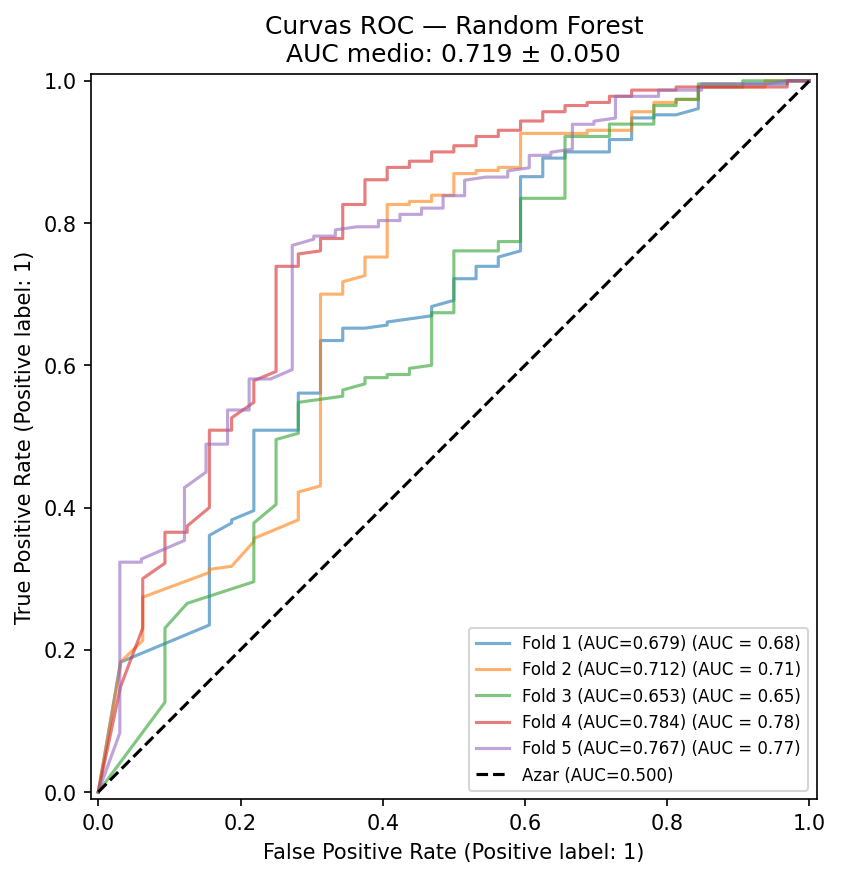
Figure 2: ROC curves from stratified cross-validation. A mean AUC-ROC of 0.719 confirms the model maintains consistent discriminative ability.
Performance analysis
The Random Forest model consistently outperformed the baselines. Although we observe a natural drop in AUC-ROC going from validation (0.72) to test (0.65), the most revealing finding lies in the predictor's reliability:
-
Perfect sensitivity (Recall = 1.0): The model detected 100% of the antigenic proteins in the test set. In a biosecurity and vaccine design context, this metric is critical: AiGenix guarantees that no potential vaccine candidate is discarded during the initial screening phase (zero false negatives).
-
High reliability (89.2% precision): With an F1-score of 0.943 on the final test, the model shows that when it flags a protein as antigenic, it's right with a very low error rate, significantly optimizing lab resources.
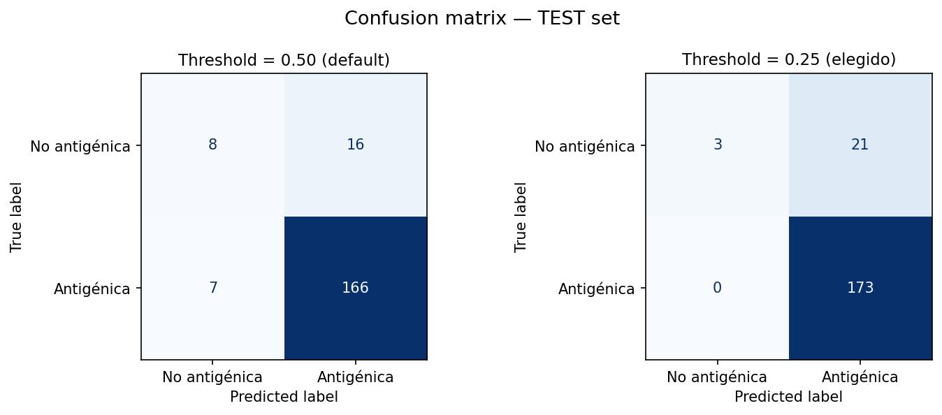
Figure 3: By setting the decision threshold to 0.25, the model maximizes recall, capturing all positives in the test set.
Feature importance and interpretation
The feature importance analysis confirms that a protein's physicochemical nature dictates its visibility to the immune system. Molecular weight and the GRAVY index (hydropathy) emerged as the strongest physical predictors.
The model "learned" biology without ever seeing 3D structures: it identified that proteins with negative GRAVY (hydrophilic) are more likely to sit on the viral surface, making them easier for antibodies to recognize.
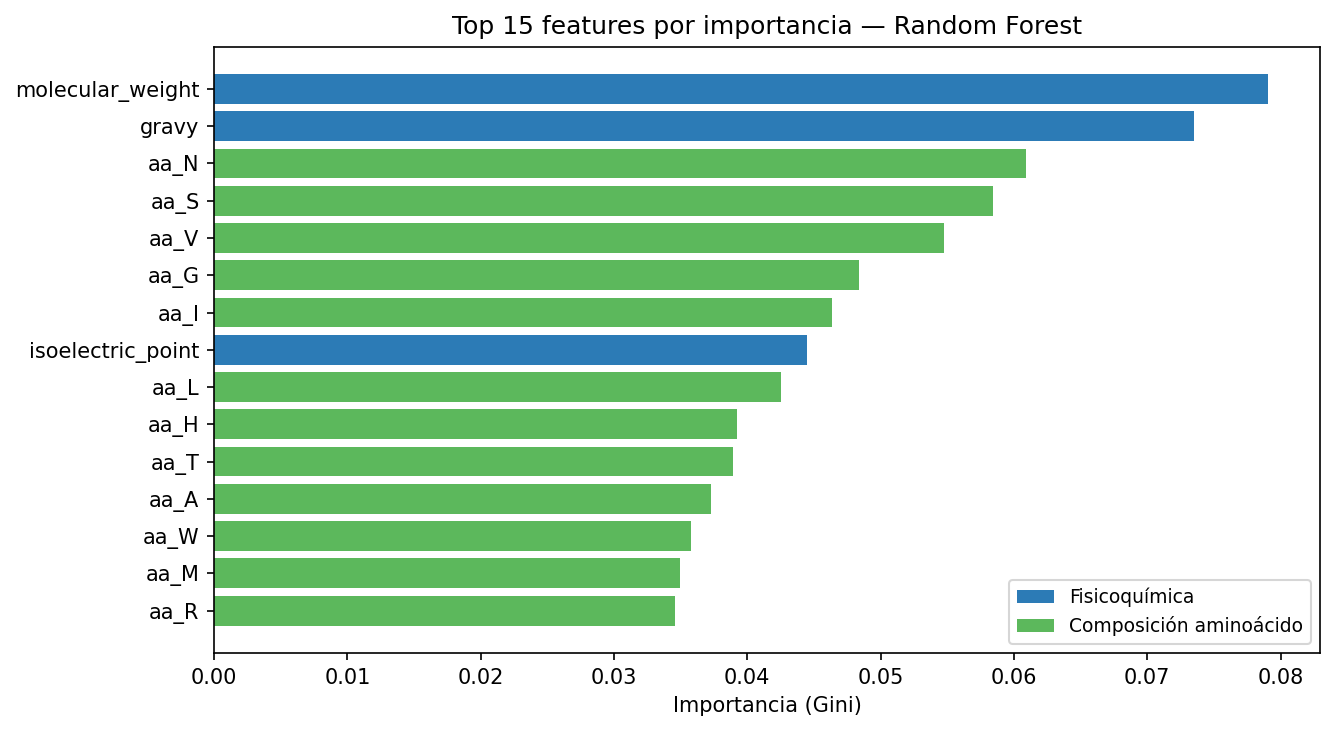
Figure 4: Molecular weight and hydropathy (GRAVY) lead the model's predictive power.
As a final proof of concept, we evaluated the structural proteins of SARS-CoV-2. The model assigned the highest probability to the Spike protein (0.830), computationally validating what the scientific community identified experimentally as the primary antigen for next-generation vaccines.
Conclusions
AiGenix demonstrates that it's possible to build a complete machine learning pipeline applied to a real biomedical problem using exclusively public data and open-source tools. The journey from 3.9 GB of lab assays to a model capable of prioritizing vaccine candidates in seconds fits into five notebooks and a few hours of compute.
But the most valuable part of the project isn't the final AUC of 0.651. It's what you learn along the way.
What works. Physicochemical sequence features capture real information about antigenicity. Achieving a Recall of 1.0 (100%) on the independent test set is the project's biggest technical win: it means AiGenix is a robust safety filter that doesn't let any potential antigen slip through. Amino acid composition, simple as it is, contains a clear biological signal that Random Forest manages to capitalize on.
What doesn't work (and why). The drop from an AUC of 0.72 in validation to 0.65 in test is a lesson in data science realism: the model faces the complexity of proteins it has never seen. This gap confirms a structural limitation: antigenicity depends critically on a protein's three-dimensional shape, not just its linear sequence. The immune system interacts with the folded surface — something our model, working with linear text, can only glimpse statistically.
About the data. The combination of perfect recall with a moderate AUC suggests that our "negative" dataset contains noise (proteins that could be antigenic but simply haven't been studied). In immunology, absence of evidence is not evidence of absence. As IEDB grows, AiGenix will be able to refine itself — but for now, we've achieved a highly effective digital "sentinel."
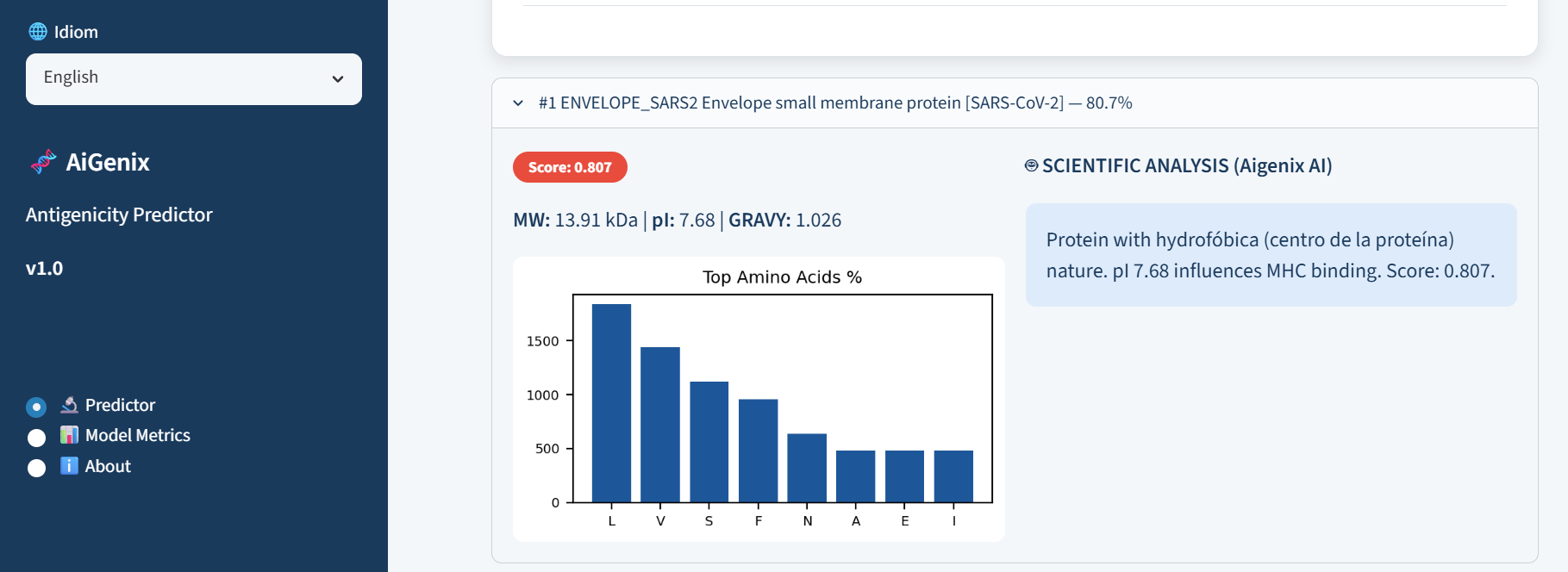
Figure 5: Explainability via generative AI. AiGenix integrates Gemini 2.0 Flash to provide the scientific reasoning behind each prediction, making biological interpretation easier.
Artificial intelligence won't replace the lab. But in a virtually infinite molecular universe, where a single pathogen can have dozens of proteins and each protein thousands of variants, helping scientists decide where to look first can make the difference between years of blind research and an early discovery.
That's what AiGenix does. It's a filter, not a verdict. And sometimes, a good filter is exactly what you need.
Code, data, and notebooks available on GitHub
A project built at Saturdays AI Madrid
Team members:
Alejandro Aparicio Calvo, Iris Fernanda Amorim, Joaquin Lazaro